library(dplyr)
library(survivoR)
## load viewer data
viewers <- survivoR::viewers |>
filter(version == "US")
## load season stats
viewers <- survivoR::viewers |>
filter(version == "US")Making survivor data
The survivoR r package has collected data about the greatest television show of all time.
To merge the castaways and castaway_details data frames from the survivoR package in R, you can follow these steps. These two data sets include different pieces of information about the contestants (castaways) of the Survivor TV show, and merging them can provide a comprehensive single dataset.
First, ensure you have the survivoR package installed and loaded along with dplyr for data manipulation:
```{r}
# Install survivoR if not already installed
if (!requireNamespace("survivoR", quietly = TRUE)) {
  install.packages("survivoR")
}

# Load necessary packages
library(survivoR)
library(dplyr)


```
Data Issues and Transformations
Descriptive Statistics
Is anyone still watching that show? Using the viewers data.
colnames(viewers)#> [1] "version" "version_season" "season"
#> [4] "episode_number_overall" "episode" "episode_title"
#> [7] "episode_label" "episode_date" "episode_length"
#> [10] "viewers" "imdb_rating" "n_ratings"glimpse(viewers)#> Rows: 701
#> Columns: 12
#> $ version <chr> "US", "US", "US", "US", "US", "US", "US", "US",…
#> $ version_season <chr> "US01", "US01", "US01", "US01", "US01", "US01",…
#> $ season <dbl> 1, 1, 1, 1, 1, 1, 1, 1, 1, 1, 1, 1, 1, 1, 2, 2,…
#> $ episode_number_overall <dbl> 1, 2, 3, 4, 5, 6, 7, 8, 9, 10, 11, 12, 13, NA, …
#> $ episode <dbl> 1, 2, 3, 4, 5, 6, 7, 8, 9, 10, 11, 12, 13, 14, …
#> $ episode_title <chr> "The Marooning", "The Generation Gap", "Quest f…
#> $ episode_label <chr> "Ep 1", "Ep 2", "Ep 3", "Ep 4", "Ep 5", "Ep 6",…
#> $ episode_date <date> 2000-05-31, 2000-06-07, 2000-06-14, 2000-06-21…
#> $ episode_length <dbl> 44, 44, 45, 45, 45, 45, 45, 45, 45, 45, 45, 45,…
#> $ viewers <dbl> 15510000, 18100000, 23250000, 24200000, 2398000…
#> $ imdb_rating <dbl> 8.0, 7.4, 7.5, 7.4, 7.3, 7.4, 7.8, 7.5, 7.5, 7.…
#> $ n_ratings <dbl> 330, 238, 229, 217, 215, 211, 210, 208, 202, 20…library(here)
library(haven)
# Set the base path for the images
base_path <- here("projects", "survivor-stats")
write_sav(viewers, here(base_path, "data", "viewers.sav"))view_data <- viewers |>
summarise(across(where(is.numeric),
list(mean = mean,
sd = sd,
median = median,
min = min,
max = max),
na.rm = TRUE))
glimpse(head(view_data))#> Rows: 1
#> Columns: 35
#> $ season_mean <dbl> 23.83595
#> $ season_sd <dbl> 13.69943
#> $ season_median <dbl> 23
#> $ season_min <dbl> 1
#> $ season_max <dbl> 48
#> $ episode_number_overall_mean <dbl> 331.5
#> $ episode_number_overall_sd <dbl> 191.2472
#> $ episode_number_overall_median <dbl> 331.5
#> $ episode_number_overall_min <dbl> 1
#> $ episode_number_overall_max <dbl> 662
#> $ episode_mean <dbl> 7.834522
#> $ episode_sd <dbl> 4.264606
#> $ episode_median <dbl> 8
#> $ episode_min <dbl> 1
#> $ episode_max <dbl> 17
#> $ episode_length_mean <dbl> 49.93866
#> $ episode_length_sd <dbl> 18.26348
#> $ episode_length_median <dbl> 43
#> $ episode_length_min <dbl> 15
#> $ episode_length_max <dbl> 130
#> $ viewers_mean <dbl> 12326877
#> $ viewers_sd <dbl> 6504079
#> $ viewers_median <dbl> 10380000
#> $ viewers_min <dbl> 4020000
#> $ viewers_max <dbl> 51690000
#> $ imdb_rating_mean <dbl> 7.559169
#> $ imdb_rating_sd <dbl> 0.6728879
#> $ imdb_rating_median <dbl> 7.6
#> $ imdb_rating_min <dbl> 4.7
#> $ imdb_rating_max <dbl> 9.5
#> $ n_ratings_mean <dbl> 150.9126
#> $ n_ratings_sd <dbl> 62.98443
#> $ n_ratings_median <dbl> 130
#> $ n_ratings_min <dbl> 16
#> $ n_ratings_max <dbl> 657view <- viewers |>
group_by(season) |>
summarize(mean = mean(viewers, na.rm = TRUE),
sd = sd(viewers, na.rm = TRUE),
n = n())
print(view)#> # A tibble: 48 × 4
#> season mean sd n
#> <dbl> <dbl> <dbl> <int>
#> 1 1 27279286. 8799047. 14
#> 2 2 29683125 4953759. 16
#> 3 3 20144000 2488260. 15
#> 4 4 20470000 3036064. 15
#> 5 5 20492000 2710889. 15
#> # ℹ 43 more rowslibrary(ggplot2)
library(scales)
library(emwthemes)
# make bar plot
p1 <- view |>
ggplot(aes(x = as.factor(season), y = mean)) +
geom_bar(stat = "identity", width = .5, fill = "tomato3") +
scale_y_continuous(
labels = scales::label_number(scale = 1e-6, suffix = "M"),
expand = expansion(mult = c(0, 0.05)), # This makes the y-axis start at 0
limits = c(0, NA) # This ensures the axis starts at 0
) +
# scale_x_discrete(guide = guide_axis(n.dodge = 2)) +
labs(title = "Ordered Bar Chart",
subtitle = "Season Vs Avg. Viewers",
caption = "source: survivoR",
x = "Season",
y = "Average Viewers (Millions)") +
theme_em() +
theme(
axis.text.x = element_text(size = 6
))
print(p1)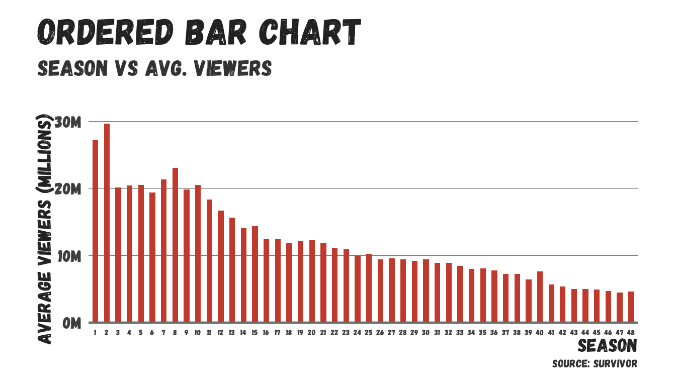
castaways <- survivoR::castaways |> filter(version == “US”)
print(castaways) details <- survivoR::castaway_details
#check the structure of the dataframes to identify which columns can be used to merge them. Ideally, find a unique identifier like an ID number colnames(castaways) colnames(details) #images <- survivoR::get_castaway_image()
Example Usage with SurvivoR Package
If you are working with a dataset from the survivoR package, such as the merged castaways and castaway_details dataframe, you can apply these methods to get more familiar with the data:
```{r}
library(survivoR)
library(dplyr)

# Assume 'merged_data' is your merged dataframe
summary(castaway_data)
str(castaway_data)
table(castaway_data$column_name)  # Replace 'column_name' with an actual column name

# Visualizations
hist(castaway_data$age)
```